scikit-learn中的多项式回归和Pipeline
1
2
| import numpy as np
import matplotlib.pyplot as plt
|
1
2
3
| x = np.random.uniform(-3, 3, size=100)
X = x.reshape(-1, 1)
y = 0.5 * x**2 + x + 2 + np.random.normal(0, 1, 100)
|
1
| from sklearn.preprocessing import PolynomialFeatures
|
1
2
3
| poly = PolynomialFeatures(degree=2)
poly.fit(X)
X2 = poly.transform(X)
|
(100, 3)
array([[ 0.14960154],
       [ 0.49319423],
       [-0.87176575],
       [-1.33024477],
       [ 0.47383199]])
array([[ 1.        ,  0.14960154,  0.02238062],
       [ 1.        ,  0.49319423,  0.24324055],
       [ 1.        , -0.87176575,  0.75997552],
       [ 1.        , -1.33024477,  1.76955114],
       [ 1.        ,  0.47383199,  0.22451675]])
1
2
3
4
5
| from sklearn.linear_model import LinearRegression
lin_reg2 = LinearRegression()
lin_reg2.fit(X2, y)
y_predict2 = lin_reg2.predict(X2)
|
1
2
3
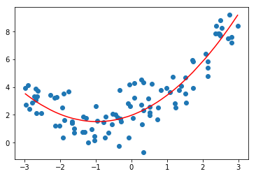
| plt.scatter(x, y)
plt.plot(np.sort(x), y_predict2[np.argsort(x)], color='r')
plt.show()
|
array([ 0. , 0.9460157 , 0.50420543])
2.1536054095953823
关于PolynomialFeatures
1
| X = np.arange(1, 11).reshape(-1, 2)
|
array([[ 1,  2],
       [ 3,  4],
       [ 5,  6],
       [ 7,  8],
       [ 9, 10]])
1
2
3
| poly = PolynomialFeatures(degree=2)
poly.fit(X)
X2 = poly.transform(X)
|
(5, 6)
array([[   1.,    1.,    2.,    1.,    2.,    4.],
       [   1.,    3.,    4.,    9.,   12.,   16.],
       [   1.,    5.,    6.,   25.,   30.,   36.],
       [   1.,    7.,    8.,   49.,   56.,   64.],
       [   1.,    9.,   10.,   81.,   90.,  100.]])
Pipeline
1
2
3
4
5
6
7
8
9
10
11
12
| x = np.random.uniform(-3, 3, size=100)
X = x.reshape(-1, 1)
y = 0.5 * x**2 + x + 2 + np.random.normal(0, 1, 100)
from sklearn.pipeline import Pipeline
from sklearn.preprocessing import StandardScaler
poly_reg = Pipeline([
("poly", PolynomialFeatures(degree=2)),
("std_scaler", StandardScaler()),
("lin_reg", LinearRegression())
])
|
1
2
| poly_reg.fit(X, y)
y_predict = poly_reg.predict(X)
|
1
2
3
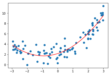
| plt.scatter(x, y)
plt.plot(np.sort(x), y_predict[np.argsort(x)], color='r')
plt.show()
|