梯度下降法和PCA

2016-07-13 机器学习 PV:

PCA和梯度法

核心思想

其实严格来说，梯度下降法不是机器学习算法，是一种基于搜索的最优方法。

主要作用是最小化一个损失函数。相对应的，梯度上升法就是最大化一个效用函数。

关于梯度下降算法的直观理解，我们以一个人下山为例。按照梯度下降算法的思想，它将按如下操作达到最低点：

第一步，明确自己现在所处的位置

第二步，找到相对于该位置而言下降最快的方向

第三步，沿着第二步找到的方向走一小步，到达一个新的位置，此时的位置肯定比原来低

第四部，回到第一步

第五步，终止于最低点

scikit-learn中使用PCA

1
2
3

import numpy as np
import matplotlib.pyplot as plt
from sklearn import datasets

1
2
3

digits = datasets.load_digits()
X = digits.data
y = digits.target

1
2
3

from sklearn.model_selection import train_test_split

X_train, X_test, y_train, y_test = train_test_split(X, y, random_state=666)

1	X_train.shape

(1347, 64)

%%time

from sklearn.neighbors import KNeighborsClassifier

knn_clf = KNeighborsClassifier()
knn_clf.fit(X_train, y_train)

CPU times: user 19.9 ms, sys: 7.47 ms, total: 27.4 ms
Wall time: 64.5 ms

1	knn_clf.score(X_test, y_test)

0.98666666666666669

from sklearn.decomposition import PCA

pca = PCA(n_components=2)
pca.fit(X_train)
X_train_reduction = pca.transform(X_train)
X_test_reduction = pca.transform(X_test)

1
2
3

%%time 
knn_clf = KNeighborsClassifier()
knn_clf.fit(X_train_reduction, y_train)

CPU times: user 2.13 ms, sys: 767 µs, total: 2.9 ms
Wall time: 2.93 ms

1	knn_clf.score(X_test_reduction, y_test)

0.60666666666666669

主成分所解释的方差

1	pca.explained_variance_ratio_

array([ 0.14566817,  0.13735469])

1	pca.explained_variance_

array([ 175.77007821,  165.73864334])

from sklearn.decomposition import PCA

pca = PCA(n_components=X_train.shape[1])
pca.fit(X_train)
pca.explained_variance_ratio_

array([  1.45668166e-01,   1.37354688e-01,   1.17777287e-01,
         8.49968861e-02,   5.86018996e-02,   5.11542945e-02,
         4.26605279e-02,   3.60119663e-02,   3.41105814e-02,
         3.05407804e-02,   2.42337671e-02,   2.28700570e-02,
         1.80304649e-02,   1.79346003e-02,   1.45798298e-02,
         1.42044841e-02,   1.29961033e-02,   1.26617002e-02,
         1.01728635e-02,   9.09314698e-03,   8.85220461e-03,
         7.73828332e-03,   7.60516219e-03,   7.11864860e-03,
         6.85977267e-03,   5.76411920e-03,   5.71688020e-03,
         5.08255707e-03,   4.89020776e-03,   4.34888085e-03,
         3.72917505e-03,   3.57755036e-03,   3.26989470e-03,
         3.14917937e-03,   3.09269839e-03,   2.87619649e-03,
         2.50362666e-03,   2.25417403e-03,   2.20030857e-03,
         1.98028746e-03,   1.88195578e-03,   1.52769283e-03,
         1.42823692e-03,   1.38003340e-03,   1.17572392e-03,
         1.07377463e-03,   9.55152460e-04,   9.00017642e-04,
         5.79162563e-04,   3.82793717e-04,   2.38328586e-04,
         8.40132221e-05,   5.60545588e-05,   5.48538930e-05,
         1.08077650e-05,   4.01354717e-06,   1.23186515e-06,
         1.05783059e-06,   6.06659094e-07,   5.86686040e-07,
         7.44075955e-34,   7.44075955e-34,   7.44075955e-34,
         7.15189459e-34])

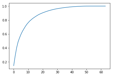
1
2
3

plt.plot([i for i in range(X_train.shape[1])], 
         [np.sum(pca.explained_variance_ratio_[:i+1]) for i in range(X_train.shape[1])])
plt.show()

png

1 2	pca = PCA(0.95) pca.fit(X_train)

PCA(copy=True, iterated_power='auto', n_components=0.95, random_state=None,
  svd_solver='auto', tol=0.0, whiten=False)

1	pca.n_components_

1 2	X_train_reduction = pca.transform(X_train) X_test_reduction = pca.transform(X_test)

1
2
3

%%time 
knn_clf = KNeighborsClassifier()
knn_clf.fit(X_train_reduction, y_train)

CPU times: user 4.21 ms, sys: 1.28 ms, total: 5.49 ms
Wall time: 19.7 ms

1	knn_clf.score(X_test_reduction, y_test)

0.97999999999999998

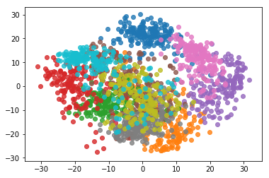
使用PCA对数据进行降维可视化

1
2
3

pca = PCA(n_components=2)
pca.fit(X)
X_reduction = pca.transform(X)

1
2
3

for i in range(10):
    plt.scatter(X_reduction[y==i,0], X_reduction[y==i,1], alpha=0.8)
plt.show()

png