scikit-learn中的SVM
1
2
| import numpy as np
import matplotlib.pyplot as plt
|
1
2
3
4
5
6
7
8
9
| from sklearn import datasets
iris = datasets.load_iris()
X = iris.data
y = iris.target
X = X[y<2,:2]
y = y[y<2]
|
1
2
3
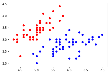
| plt.scatter(X[y==0,0], X[y==0,1], color='red')
plt.scatter(X[y==1,0], X[y==1,1], color='blue')
plt.show()
|
1
2
3
4
5
| from sklearn.preprocessing import StandardScaler
standardScaler = StandardScaler()
standardScaler.fit(X)
X_standard = standardScaler.transform(X)
|
1
2
3
4
| from sklearn.svm import LinearSVC
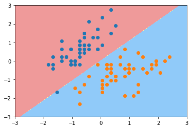
svc = LinearSVC(C=1e9)
svc.fit(X_standard, y)
|
LinearSVC(C=1000000000.0, class_weight=None, dual=True, fit_intercept=True,
     intercept_scaling=1, loss='squared_hinge', max_iter=1000,
     multi_class='ovr', penalty='l2', random_state=None, tol=0.0001,
     verbose=0)
1
2
3
4
5
6
7
8
9
10
11
12
13
14
15
| def plot_decision_boundary(model, axis):
x0, x1 = np.meshgrid(
np.linspace(axis[0], axis[1], int((axis[1]-axis[0])*100)).reshape(-1, 1),
np.linspace(axis[2], axis[3], int((axis[3]-axis[2])*100)).reshape(-1, 1),
)
X_new = np.c_[x0.ravel(), x1.ravel()]
y_predict = model.predict(X_new)
zz = y_predict.reshape(x0.shape)
from matplotlib.colors import ListedColormap
custom_cmap = ListedColormap(['#EF9A9A','#FFF59D','#90CAF9'])
plt.contourf(x0, x1, zz, linewidth=5, cmap=custom_cmap)
|
1
2
3
4
| plot_decision_boundary(svc, axis=[-3, 3, -3, 3])
plt.scatter(X_standard[y==0,0], X_standard[y==0,1])
plt.scatter(X_standard[y==1,0], X_standard[y==1,1])
plt.show()
|
1
2
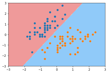
| svc2 = LinearSVC(C=0.01)
svc2.fit(X_standard, y)
|
LinearSVC(C=0.01, class_weight=None, dual=True, fit_intercept=True,
     intercept_scaling=1, loss='squared_hinge', max_iter=1000,
     multi_class='ovr', penalty='l2', random_state=None, tol=0.0001,
     verbose=0)
1
2
3
4
| plot_decision_boundary(svc2, axis=[-3, 3, -3, 3])
plt.scatter(X_standard[y==0,0], X_standard[y==0,1])
plt.scatter(X_standard[y==1,0], X_standard[y==1,1])
plt.show()
|
array([[ 4.03243305, -2.49295041]])
array([ 0.9536471])
1
2
3
4
5
6
7
8
9
10
11
12
13
14
15
16
17
18
19
20
21
22
23
24
25
26
27
28
29
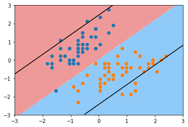
| def plot_svc_decision_boundary(model, axis):
x0, x1 = np.meshgrid(
np.linspace(axis[0], axis[1], int((axis[1]-axis[0])*100)).reshape(-1, 1),
np.linspace(axis[2], axis[3], int((axis[3]-axis[2])*100)).reshape(-1, 1),
)
X_new = np.c_[x0.ravel(), x1.ravel()]
y_predict = model.predict(X_new)
zz = y_predict.reshape(x0.shape)
from matplotlib.colors import ListedColormap
custom_cmap = ListedColormap(['#EF9A9A','#FFF59D','#90CAF9'])
plt.contourf(x0, x1, zz, linewidth=5, cmap=custom_cmap)
w = model.coef_[0]
b = model.intercept_[0]
plot_x = np.linspace(axis[0], axis[1], 200)
up_y = -w[0]/w[1] * plot_x - b/w[1] + 1/w[1]
down_y = -w[0]/w[1] * plot_x - b/w[1] - 1/w[1]
up_index = (up_y >= axis[2]) & (up_y <= axis[3])
down_index = (down_y >= axis[2]) & (down_y <= axis[3])
plt.plot(plot_x[up_index], up_y[up_index], color='black')
plt.plot(plot_x[down_index], down_y[down_index], color='black')
|
1
2
3
4
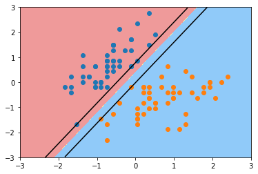
| plot_svc_decision_boundary(svc, axis=[-3, 3, -3, 3])
plt.scatter(X_standard[y==0,0], X_standard[y==0,1])
plt.scatter(X_standard[y==1,0], X_standard[y==1,1])
plt.show()
|
1
2
3
4
| plot_svc_decision_boundary(svc2, axis=[-3, 3, -3, 3])
plt.scatter(X_standard[y==0,0], X_standard[y==0,1])
plt.scatter(X_standard[y==1,0], X_standard[y==1,1])
plt.show()
|